
1 Introduction
In recent years, with the development of the flow metering industry, electromagnetic flow meters have been applied to various occasions due to their advantages of no moving parts, no pressure loss, and wide measurement range, and a problem encountered in the use process is how to improve. Large diameter large flow meter accuracy. If a pipeline-type electromagnetic flowmeter is used to measure the flow rate of a large-diameter pipe, the volume is large, the processing cost is high, calibration and installation and maintenance are very difficult, and it brings a lot of inconvenience to the engineering application. Therefore, in this case, a plug-in electromagnetic flowmeter is generally used instead of a pipeline-type electromagnetic flowmeter to measure the flow of a large-diameter pipe.
However, plug-in electromagnetic flowmeters produce nonlinear phenomena that affect the accuracy of the measurement. Many scholars now solve this problem by using a multi-stage linear compensation method. The flow within the entire measurement range is divided into multiple flow segments, and then the flow coefficients in different phases are solved to obtain the flow values ​​for each segment. However, this method is more complicated to use and its accuracy is limited. Therefore, starting from the structure of the electromagnetic flowmeter itself, this paper identifies the causes of the non-linear phenomenon, and finds a way to increase the linearity of the plug-in electromagnetic flowmeter from the source.
2 plug-in electromagnetic flowmeter working principle
Plug-in electromagnetic flowmeter measuring principle is based on Faraday's law of electromagnetic induction
 (1)
(1)
Among them, E is the induced electromotive force generated between the two electrodes, B is the magnetic induction intensity, L is the effective length of the cutting magnetic induction line, ç‹v is the average flow rate, and the fluid is the conductive medium. The schematic diagram is shown in FIG. 1 .
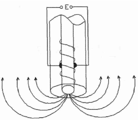
Figure 1 plug-in electromagnetic flowmeter schematic
And (1) can be expressed as
 (2)
(2)
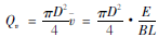
When both B and L are constant, as long as the induced electromotive force E is measured, the average flow rate can be obtained.  Because the cross-sectional area of ​​the pipeline under test is known, it is easy to determine the volumetric flow of a conductive fluid.
 (3)
(3)
Among them, D is the inner diameter of the measured pipe, Qv is the volume flow.
From the formula (3), it can be seen that when the insertion pipe structure is certain, the volumetric flow rate Qv is proportional to the ratio E/B, and is independent of the fluid temperature, density, and pressure inside the pipe. When the magnetic induction B is constant, the volumetric flow rate Qv is proportional to the induced electromotive force E, that is, the volume flow rate and the induced electromotive force are completely linear.
3 sensor linearity assessment
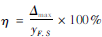
Linearity is one of the main static performance indicators of a sensor. It is defined as a measure of whether a test system's output and input system can maintain a normal ratio (linear relationship) as an ideal system. Linearity reflects the degree to which the calibration curve agrees with a given straight line, which is an ideal straight line determined by a certain method. Linearity, also known as nonlinearity, refers to the linearity definition in GB/T18459-2001 "Calculation Method for Primary Static Performance of Sensors": Actual and Backward Travel Actual Mean Characteristic Curve Relative to Reference Line (Line Fit) Deviation, expressed as a percentage of full-scale output. This indicator is usually expressed as a linear error
 (4)
(4)
Among them, Δmax is the residual, and yF.S is the theoretical full-scale output.
This paper uses the least squares method to evaluate the linearity, that is, the fitting straight line is the least squares straight line. The least-squares straight line guarantees that the average of the actual output of the sensor is the minimum of the square of its deviation, that is, the deviation between the result obtained by fitting the straight line and the measured result can be guaranteed to be small and more reliable. By definition, linearity is the degree to which the calibration curve deviates from this least-squares fit line.
4 Plug-in electromagnetic flowmeter causes non-linear phenomenon
The plug-in electromagnetic flowmeter is used for punching and inserting in the appropriate position of the pipeline under test to measure the flow of the conductive fluid, and can be taken out under constant flow for cleaning and maintenance, and the operation is very convenient. However, the probe inserted into the pipeline is equivalent to the introduction of a choke device to the flow field of the pipeline. The fluid moves around this probe, as shown in Figure 2.
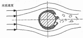
Figure 2 Flow around the probe
As fluid flows around the probe, a boundary layer forms on the probe surface due to the presence of viscous forces. As the fluid flows up and down along the curved surface, the thickness of the boundary layer increases. The closer to the wall, the more complicated the flow field changes. The change in the flow field distribution will increase the error between the measured average flow velocity and the actual flow velocity. And when the reverse pressure gradient is large enough, backflow will lead to the separation of the boundary layer, and the formation of wake vortex, that is, the separation of the boundary layer, which will increase the nonlinear phenomenon. That is, the non-linearity between the measured average flow velocity and the incoming flow velocity leads to the destruction of the linear relationship between the induced electromotive force and the measured flow, and the accuracy of the plug-in electromagnetic flowmeter measurement is reduced.
There are many factors that affect this linear relationship, mainly the plug-in electromagnetic flowmeter installation angle, insertion depth, probe shape and so on. The effect of mounting angle and insertion depth on the linear relationship between the input and output signals can be eliminated by properly installing the flow meter and calibration experiments. Therefore, the reason for the linearity of the plug-in electromagnetic flow meter studied in this paper is mainly the shape of the probe inserted into the pipe. The influence of different probe shapes on the flow field distribution in the pipe is not the same.
In this paper, FLUENT software is used to simulate the influence of four different shapes of insert probes on the flow field of the pipeline. In the range of 0.5m/s to 15m/s, several typical speed points are selected as the entrance velocity, perpendicular to the The mean flow velocity of the cross-section of the two electrodes in the direction of the incoming flow was taken as the average velocity of the signal collected, and the relationship between them was obtained by fitting. According to the comparison of the deviation between the flow velocity and the actual flow rate obtained by comparing the least squares fitting straight lines obtained under different shapes of the probes, the linearity is judged to be good or bad, so that a linearity probe type can be obtained.
5 Numerical Model Design
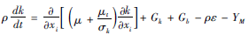
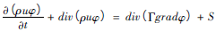
In this paper, the pre-processing software GAMBIT is used to construct the four common types of plug-in electromagnetic flowmeter probes in engineering, as shown in Figure 3. The inner diameter of the pipe is set to 400mm, the insertion depth is 120mm, the probe radius is 32mm, and the electrode radius is 5mm.
5.1 Turbulence Model
The turbulence model in this paper uses the most widely used standard k-ε model in engineering and requires solving the turbulent kinetic energy and its dissipation rate equation. In this model, the transport equations for the turbulent kinetic energy k and the dissipation rate ε are as follows
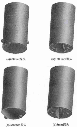
Figure 3 four kinds of probe shape
 (5)
(5)
 (6)
(6)
Among them, the turbulent viscosity coefficient  , kinetic energy
 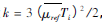 Dissipation rate
  = 1.0, σε = 1.3.
5.2 Grid Division
The GAMBIT software is used to mesh the flow field. Because the three-dimensional flow field calculation area is to be simulated, it is also necessary to make the operation as simple as possible in the premise of ensuring the accuracy. Therefore, a close-knit mesh is formed near the area around the probe. The grid, and relatively thin grids are divided in the area of ​​the straight pipe before and after to meet the calculation requirements. The mesh format unit used in this paper is Tet/Hybrid, and the specified format type is TGrid, which indicates that the specified mesh is mainly composed of a tetrahedral mesh, but may contain hexahedral, pyramidal, and wedge-shaped mesh cells in place.
5.3 Establish Discretization Equation
This paper uses the most widely used finite volume method in engineering today to divide the computational area into a series of control volumes and integrate the differential equations for each control volume to obtain the discrete equations. Universal conservation equations for solving mass, momentum, energy, composition, etc. on these controllers
 (7)
(7)
Among them, the first item on the left is a transient item, the second item is a convection item, the first item on the right is a diffusion item, and the second item is a general source item. The φ in the equation is a generalized variable and can represent some physical quantities such as velocity, temperature, pressure, etc. to be solved. Γ is the generalized diffusion coefficient corresponding to φ. The boundary value of the variable φ at the endpoint is known.
The SIMPLE algorithm is used in the control equation and belongs to the pressure correction method. The second-order upwind style is used to make the calculation result more accurate.
5.4 Determining Boundary Conditions
Experiments were carried out under the conditions of normal temperature and pressure (20°C, 1 atm) as the influent fluid. The inlet boundary condition of the pipeline was set as the velocity inlet, and the boundary condition of the pipeline outlet was the pressure outlet. Select the following 8 speed points for simulation: 0.5m/s, 1.0m/s, 2.5m/s, 5m/s, 7.5m/s, 10m/s, 12.5m/s, 15m/s, observe the flow field Distribution, you can get the average flow rate of the signal collected.
Product categories of High Pressure Cleaning Equipment, we are specialized manufacturers from China, High Pressure Plunger Pumps, High Pressure Pumps suppliers/factory, wholesale high-quality products of Triplex Pumps R & D and manufacturing, we have the perfect after-sales service and technical support. Look forward to your cooperation!
Widely used in Car cleaning,The sewer dredging,Markets & Applications,Commercial Contractor Cleaning,Vehicle Cleaning,Process Industries
Cleaning Equipment,Car Washer,Pressure Washer,High Pressure Washing Cleaner,Cleaning Machine,High Pressure Cleaner,Gasoline Washer,Petrol Cleaner,Petrol Engine High Washing,Automotive Washing Machines
Zhejiang Botuolini Machinery Co.,Ltd , https://www.chinaplungerpump.com